Showing posts with label solar energy. Show all posts

Sunday, 7 July 2024

Visualising NREL's Annual Technology Baseline ("ATB") data for wind and solar energy using R

In the US, the Federal Government's National Renewable Energy Lab released the 2024 "Annual Technology Baseline" a couple of weeks ago. The large, yearly dataset does a few things. For one, it collects data on constructed electricity generators by type of fuel/renewable and collates the components of their cost. By factoring in all of the expected outlays for a specific type of generator, we can arrive at the "Levelised Cost of Energy" (LCOE); the exact calculation can differ but essentially, the units of the LCOE are "units of currency for a unit of energy," eg, $/MWh. This allows people to ask clear, quantified questions of the type "Which type of energy generation is more (less) expensive?". In general, I have been used to calculating LCOE as a lifetime cost, but I should point out that the calculation used by NREL (see here) is a bit different than myself and most others (I believe) might have used, and it varies by year. 


 For people interested in intermittent renewables like solar and wind, NREL data also divides regions into categories defined by the strength of their wind or solar resources, on a 1 to 10 scale (1 being best and 10 being least good). These categories are defined by NREL here for solar and here for wind--note that the wind categorisation has implications for the hub height of the wind turbines to be used. 

I wanted to be able to think of a state at random within the US and ask "In which counties would I have the best (or worst?) opportunities to build a solar farm and/or a wind farm?". To do this, I would need to be able to tie climatology data (from our trusty friend nasapower) and categorise it based on the system devised by NREL. Using the R "simple features" object type, it's possible to transform this into easily readable maps, too. 


Where in Arizona do wind turbines cost the least (the most) to operate?


The way in which I've written the scripts gives users the choice between Canada, the United States and Mexico--but this is may be a flurry on my part, since NREL bases its ATB data on findings from projects in the contiguous 48 states. In the meantime, it's possible that these scripts could be built on to cover the world more globally (see below). 

There are a number of ways this project can be made better, including, to wit: 

  1. Expanding the data sources to cover a greater number of countries 
  2. Factoring in the grid connection costs, a major obstacle for renewables projects but which do not form a part of the LCOE
  3. Allowing a different calculation of the LCOE

I made the scripts available on my GitHub, here. To run this locally on your machine, all you would need is to have R installed; the "quick_start" script pretty much takes care of the rest (I tested this using R Studio, but I don't see why you couldn't use them witg the console).

Wednesday, 12 May 2021

Follow-up: Second Outtake on Calgary RUG Meeting on 21 April

So I was originally hoping to get this one out of the way before 21 April when I spoke to the Calgary R Users' Group. If you want to see me deliver the talk, complete with unkempt beard and wild shirt, here it is:
Before I say anything else: there must be thousands of RUGs across the world, but I do imagine that the Calgary RUG is one of the best. They are a dedicated, serious and hardworking bunch who also don't take themselves so seriously. You can keep up with them here: https://www.meetup.com/calgaryr/

For the matter at hand, here's a second "out take" from the talk, where I explain how to create a map which labels cities across the world with dots corresponding in size to their annual solar radiation.
By the time you're done, you should have a map which looks like this one here.

Have fun!
#To get the longitude, latitude for the cities in question, you will need to install nominatim for Open Street Maps
#devtools::install_github("hrbrmstr/nominatim")
# You will ned an OSM API key which you can get for free from Map Quest 
# Then you just populate the data frame like so 

calgary.rug.cities = c("Calgary", "Vancouver", "Edmonton", "Yellowknife", "Winnipeg", "Utrecht", "Buenos Aires", "Ramallah", "Doha", "Berlin")
calgary.rug.countries = c("CA", "CA", "CA", "CA", "CA", "NL", "AR", "PS", "QA", "DE")
#You need to know the ISO country codes for the countries in question, I suppose 


calgary.rug.solar.df = data.frame(matrix(nrow = length(calgary.rug.cities), ncol = 2))
for(i in 1:length(calgary.rug.cities))
{
  place_holder = nominatim::osm_geocode(query = calgary.rug.cities[i], country_codes = calgary.rug.countries[i], key = myosmapikey)
  calgary.rug.solar.df[i,1] = place_holder$lon
  calgary.rug.solar.df[i,2] = place_holder$lat
  print("One more city")
}
#We will need 13 columns of insolation data, one for each month and one for the annual values
calgary.rug.solar.monthly = data.frame(matrix(nrow = nrow(calgary.rug.solar.df), ncol = 13))
for(i in 1:nrow(calgary.rug.solar.monthly))
{
  request_solar_ghi = nasapower::get_power(community = "SSE", pars = "ALLSKY_SFC_SW_DWN", temporal_average = "CLIMATOLOGY", lonlat = c(calgary.rug.solar.df[i,1], calgary.rug.solar.df[i,2]))
  #To see how this next line works, you really have to know what the structure of the returned response from NASAPOWER
  calgary.rug.solar.monthly[i,] = data.frame(request_solar_ghi[which(request_solar_ghi$PARAMETER == "ALLSKY_SFC_SW_DWN"),][,4:16])
}
colnames(calgary.rug.solar.monthly) = colnames(data.frame(request_solar_ghi[,4:16]))
#Check this to see what it is
calgary.rug.solar.monthly
rownames(calgary.rug.solar.monthly) = calgary.rug.cities
calgary.rug.solar.df = cbind(calgary.rug.solar.df, calgary.rug.solar.monthly$ANN)
calgary.rug.solar.df
row.names(calgary.rug.solar.df) = calgary.rug.cities
colnames(calgary.rug.solar.df) = c("LON", "LAT", "Annual GHI")
calgary.rug.solar.df

#The annual value is given as a "average day," so we need to fix it 
calgary.rug.solar.df$`Annual GHI` = calgary.rug.solar.df$`Annual GHI`*365
calgary.rug.solar.df

calgary.rug.cities.diffuse = vector(length = length(calgary.rug.cities))
for(i in 1:length(calgary.rug.cities.diffuse))
{
  diffuse_request = nasapower::get_power(community = "SSE", pars = "DIFF", temporal_average = "CLIMATOLOGY", lonlat = c(calgary.rug.cities.for.presenting$LON[i], calgary.rug.cities.for.presenting$LAT[i]))
  annual_diffuse = data.frame(diffuse_request)$ANN
  calgary.rug.cities.diffuse[i] = annual_diffuse
}

calgary.rug.cities.dnr = vector(length = length(calgary.rug.cities))
for(i in 1:length(calgary.rug.cities))
{
  dnr_request = nasapower::get_power(community = "SSE", pars = "DNR", temporal_average = "CLIMATOLOGY", lonlat = c(calgary.rug.cities.for.presenting$LON[i], calgary.rug.cities.for.presenting$LAT[i]))
  annual_dnr = data.frame(dnr_request)$ANN
  calgary.rug.cities.dnr[i] = annual_dnr
}

calgary.rug.cities.diffuse[is.na(calgary.rug.cities.diffuse)] <- 0
calgary.cities.diff_to_dnr = calgary.rug.cities.diffuse/calgary.rug.cities.dnr

#Yelloknife is a special case it seems; just not a lot of sunlight in some parts of the year 
calgary.rug.yellowknife_diffuse1 = data.frame(nasapower::get_power(community = "SSE", pars = "DIFF", temporal_average = "CLIMATOLOGY", lonlat = c(calgary.rug.cities.for.presenting$LON[4], calgary.rug.cities.for.presenting$LAT[4])))
calgary.rug.yellowknife_diffuse = sum((calgary.rug.yellowknife_diffuse1)[,4:16], na.rm = TRUE)
calgary.rug.yellowknife_dnr1 = data.frame(nasapower::get_power(community = "SSE", pars = "DNR", temporal_average = "CLIMATOLOGY", lonlat = c(calgary.rug.cities.for.presenting$LON[4], calgary.rug.cities.for.presenting$LAT[4])))
calgary.rug.yellowknife_dnr = sum(calgary.rug.yellowknife_dnr1[,4:16], na.rm = TRUE)
calgary.rug.yellowknife_diff_to_dnr = calgary.rug.yellowknife_diffuse/calgary.rug.yellowknife_dnr
calgary.cities.diff_to_dnr[4] = calgary.rug.yellowknife_diff_to_dnr

calgary.rug.cities.for.presenting$DiffDNR = calgary.cities.diff_to_dnr


#Before going any further, please have a quick check to see that the different data frames are reasonable before trying to plot them

myPaletter = colorRampPalette(rev(brewer.pal(11, "RdBu")))
scaled_map = scale_color_gradientn(colors = myPaletter(25), limits = c(min(calgary.rug.solar.df$DiffDNR2), max(calgary.rug.solar.df$DiffDNR2)), name = "Diffuse-to-DNR \n %-age")


#The map for diffuse to DNI 
ggplot2::ggplot(data = world_map) +
  geom_sf() +
  geom_point(data = calgary.rug.solar.df[1:10,],
             mapping = aes(x = LON, y = LAT,
                           color = (DiffDNR2)),
             size = 5) +   coord_sf(xlim = c(min(calgary.rug.cities.for.presenting$LON)-10,
                                             max(calgary.rug.cities.for.presenting$LON) + 10),
                                    ylim = c(min(calgary.rug.cities.for.presenting$LAT)-10,
                                             max(calgary.rug.cities.for.presenting$LAT)+10), expand = F) +
  scaled_map +
  ggtitle("Diffuse to DNR annually \n selected cities") +theme(panel.background = element_rect(fill = "lightblue",  color = "blue", size = 0.5))

Thursday, 11 March 2021

"The Alberta Albedo Advantage", or "Why my transitions always darken in Alberta"

Before moving on to the final part of this series on solar irradiance and solar PV power across Alberta, I wanted to do a little segway and talk about how albedo is a particularly relevant issue for the workings of PV panels in Alberta and similar places. This is also in part a short elaboration/commentary on a presentation I heard as part of a webinar organised by Solar Alberta on February 25.


Let me say: if you'd rather just jump to the bit which has R codes to download the relevant data, then please just click here . If you're wondering what albedo is, please read on.

In the earlier blog post, what I did was to model the amount of solar insolation at a given site through the "Global Horizontal Irradiation," or GHI, which is a measure of the amount of solar energy that falls on a horizontally flat solar panel that is "looking up". GHI is in turn made up of two separate components. The larger of these is the component of the solar insolation which falls more or less straight down, also known as Direct Normal Irradiance or "DNI". A second component however is made up of the solar insolation which hits the panel after bouncing off of the atmosphere and, especially in the case of PV panels deployed in urban settings, of large, reflective structures.
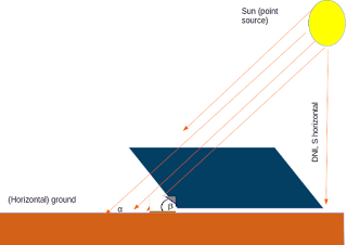


Finally, it's worth considering also what happens when the solar PV panel is--as is typical--tilted. In that case, the total solar irradiation on the PV panel--in the "plane of array"--is the sum of three distinct components, one of which is the component which falls directly on the panel in a normal from the sun; a second component which is diffuse solar radiation from the atmosphere and which lands on the tilted panel; and a third component which is reflected off of the ground and meets the panel. Programmatically, this is just: 


Gtotal = GDNI + GDIFF + Gground
A really good way to understand these different components is to read the explanations of various (competing) models of POA irradiance models on the Sandia website. For my purposes, I will use the following conversions:
Beam irradiance, GBeam
The beam irradiance is a product of the cosine of the tilt angle (θ) and the DNI: Gbeam = GDNI *cos(θ)
Ground reflected component, GGround
The ground reflected component is going to similarly be a function of the tilt angle but also an "albedo" constant, ρ ,which we can quantify for each month at each location. Note the definition of albedo right there: it's simply a two-dollar word for how much light is reflected off a particular piece of ground. GHI * ρ * 1 - cos(θ) 2
Diffuse component, GDIFF
Let me just refer you back to the Sandia website. I'll be frank, there are too many competing models to compute how much solar irradiance is diffuse in the atmosphere above a certain site at a given time, and I'd rather just focus on crunching out the numbers for this blog post. I will simply download the diffuse irradiance below.

Let me just point out, once again: it's important not to confuse the GHI and DNI types of irradiance. The latter is the bit which falls directly downwards on a flat solar PV panel, while the former includes other components.
Also, you're possibly wondering about the full title of this blog post. Here's a picture of my transition type glasses which I took on my Edmonton balcony the other (not very sunny) day. What could the fact of the transitions having faded to black on a not-so-sunny day got to do with solar PV electricity and its availability? Quite a lot!

Finally, before moving on to the R code, I should probably point out that we will make use of a specific way to calculate the tilt angle. As with so many things, there are multiple approaches to calculating a tilt angle, which in general factor in the latitude of a given location and a temporal factor. Depening on your desired level of exactness, this temporal factor can vary from month, day or even hour: it is meant to account for the changes in the solar azimuth angle and the location of the PV panel. You can find papers which compare multiple models for calculating the optimal tilt angle for a given location, such as this one from Palestine. For Western Canada--which we've defined here as just the provinces of British Columbia and Alberta--the latitudes range from 48.56 to 59.07, measuring roughly 1100 kms North-South. Figuring out a specific tilt angle for each location within our dataset, while more "correct," might not be a great use of time for a simple blog post.
One perfectly reasonable compromise I can find is to use the approach in Stanicu and Stanicu, which is to define the tilt angle θ as the sum of the latitude, φ and declination angle, δ : θ = φ + δ
For its part, the declination angle is a function of the day of the year, d:
δ = -23.45*cos(0.986*(d+10))
In a later part of this post, I will show how this can be coded into R.

The R Codes

From here on, I'm just going to focus on the mechanics of downloading the data and presenting it in the same way as I did last time. Once finished, I will show how albedo--due largely to snow cover--makes the question of solar insolation and, eventually, PV electricity, in Alberta more nuanced than would be thought about if all you did is look at GHI.
In the next code snippet, I am going to first load all of the R packages I need and then move on from there to add names to the "Census Divisions" in Alberta.
library(rgeos)
library(maptools)
library(ggmap)
library(ggplot2)
library(sp)
library(rgdal)
library(raster)
library(nasapower)
library(scales)
library(plyr)

alberta_division_names = c("Medicine Hat", "Lethbridge", "Claresholm", "Hanna", "Strathmore", "Calgary", "Wainwright", "Red Deer", "Rocky Mountain House", "Lloydminster", "Edmonton", "Cold Lake", "White Court", "Hinton", "Canmore", "Fort McMurray", "Slave Lake", "Grande Cache", "Grande Prairie")
#We want to be able to combine/compare these with the districts in British Columbia 
western_canada_province_names = western_canada_ellipsoid@data$NAME_1
western_canada_division_names = c(alberta_division_names, western_canada_ellipsoid@data$NAME_2[20:47])

western_canada_district_names = c(alberta_division_names, western_canada_ellipsoid@data$NAME_2[20:47])
western_canada_albedo_annual = cbind(western_canada_district_names, western_canada_albedo_monthly[,13])


Next, one straightforward thing is to use nasapower to download values for the diffuse solar irradiation and also the surface albedo constant. The "parameter," or keyword, which nasapower uses to define these values are "DIFF" and "SRF_ALB", and to turn these into dataframes. As always, I am using the "CLIMATOLOGY" timeframe which takes monthly averages for the period between 1984 and 2013 and the "SSE" community which specifies that the units used will be useful for the renewable energy community. In the code snippet below: I create distinct data.frame objects which cover all of the sets of data that we want. Unlike in the previous post, I am just going to treat "Western Canada" as one single unit here and from there . I download both sets of data for each site in our dataset. From there, I divide each request from the server into separate data.frame. Finally, I populate each row of the dedicated data frames with the relevant retrieved data.
One thing you'll notice is that I do two separate requests: one for the GHI alone and one for the albedo, DNI/DNR and Diffuse components combined. This is purely because the API request only allows a maximum of three parameters to be downloaded at once if you're using the "CLIMATOLOGY" timeframe. Next, I should point out that while I also downloaded GHI radiation last time, that was limited to using annual values. Later on, it will become clear why monthly data are also valuable for this blog post.
#We want four types of data on a monthly basis for each site: albedo constants as well as GHI, DNR (aka DNI) and Diffuse insolation
western_canada_dnr_monthly = data.frame(matrix(ncol = 13, nrow = nrow(western_canada_coordinates)))
western_canada_ghi_monthly = data.frame(matrix(ncol = 13, nrow = nrow(western_canada_coordinates)))
western_canada_albedo_monthly = data.frame(matrix(ncol = 13, nrow = nrow(western_canada_coordinates)))
western_canada_diffuse_monthly = data.frame(matrix(ncol = 13, nrow = nrow(western_canada_coordinates)))
                                           
for(i in 1:nrow(western_canada_coordinates))
{
  #Get the data from NASA POWER
  #Make sure to use the correct parameter names from nasapower
  #retrieved_parameters = nasapower::get_power(community = "SSE", pars = c("DNR",  "DIFF","SRF_ALB"), lonlat = c(western_canada_coordinates[i,1],
                                                                                   
  #See the explanation above for why we do this with two requests                                                                                                                                                        western_canada_coordinates[i,2]), temporal_average = "CLIMATOLOGY")
  retrieved_global_horizontal = nasapower::get_power(community = "SSE", pars ="ALLSKY_SFC_SW_DWN", lonlat = c(western_canada_coordinates[i,1],
                                                                                                                                    western_canada_coordinates[i,2]), temporal_average = "CLIMATOLOGY")
  #Split the API request into separate data.frames
  #Notice that the original request returns a tibble, which is more information than we want/need
  #Once we divide it into 4 data.frames, we fill one row of each of the data.frames we want
  retrieved_albedo = data.frame(retrieved_parameters[which(retrieved_parameters$PARAMETER == "SRF_ALB"),])
  retrieved_diffuse = data.frame(retrieved_parameters[which(retrieved_parameters$PARAMETER == "DIFF"),])
  retrieved_dnr = data.frame(retrieved_parameters[which(retrieved_parameters$PARAMETER == "DNR"),])
  retrieved_ghi = data.frame(retrieved_global_horizontal[which(retrieved_global_horizontal$PARAMETER == "ALLSKY_SFC_SW_DWN"),])
  #Since we've set up data.frames for the information/data we need, populate each row of those two data.frames
  western_canada_albedo_monthly[i,] = retrieved_albedo[,4:16]
  western_canada_diffuse_monthly[i,] = retrieved_diffuse[,4:16]
  western_canada_dnr_monthly[i,] = retrieved_dnr[,4:16]
  western_canada_ghi_monthly[i,] = retrieved_ghi[,4:16]
  #Just a quick check 
  print(paste("Ya habeebi, we are at site", i, sep = ", "))
}

We now have monthly averages for the DNR, the Albedo constant and the diffuse irradiation/insolation for each of the 47 Level 2 districts in Western Canada. As with the previous post, the data is gathered based on the longitude and latitude coordinates of the centroids of each district, using the NASA POWER package from Cran. Doubtlessly, using the centroids for each of these districts is probably introducing at least some kind of errors--you wouldn't necessarily want to place solar panels there unless you've determined that doing so is coincidentally the optimal location for solar radiation. I might re-visit this in a later blog spot, but for now this will do. One thing which I never quite liked but have found efficient is the very "tight" syntax for subsetting data.frames: your_subset = your_data_frame[which(your_data$COLUMN_NAME == "your criterion",)]. If you're confused about why I chose columns 4:16, please see the previous post.
How to compute the tilt angles per site per month? In the snippet below, I define what the "median day" per month is. I then calculate straight away what the tilt angle is for that median day.

days_in_months = c(31, 28, 31, 30, 31, 30, 31, 31, 30, 31, 30, 31)
#Now we want is to know what the median number of days 
midpoint_of_months =  ceiling(0.5*days_in_months)
#Now, to find the median day of each month as out of the day 
cumulative_days_months = cumsum(days_in_months)
median_days_of_months = vector(length = 12)
median_days_of_months[1] = midpoint_of_months[1]
for(i in 2:12)
{
  #We start with the previous month and then add to it to the median number
  #of days from the present month 
  median_days_of_months[i] = cumulative_days_months[i-1] + midpoint_of_months[i]
}

It's important to make clear that R computes trignometric functions using radians while so far we've been assuming that it's degrees. Below, I create a simple function which turns degrees into radians and then finally returns a monthly tilt angle for each of the Level 2 sub-divisions in Western Canada.
#Make a function that takes degrees and returns radians
deg_to_rad <- function(degrees)
{
  rads_to_return = degrees*pi/180
  return(rads_to_return)
}

#Defining the declination angles 
#Define the number of days per month 
days_in_months = c(31, 28, 31, 30, 31, 30, 31, 31, 30, 31, 30, 31)
#Now we want is to know what the median number of days 
midpoint_of_months =  ceiling(0.5*days_in_months)
#Now, to find the median day of each month as out of the day 
cumulative_days_months = cumsum(days_in_months)
median_days_of_months = vector(length = 12)
median_days_of_months[1] = midpoint_of_months[1]
for(i in 2:12)
{
  #We start with the previous month and then add to it to the median number
  #of days from the present month 
  median_days_of_months[i] = cumulative_days_months[i-1] + midpoint_of_months[i]
}

#Declination angles, change only by month
declinations_monthly = vector(length = 12)
for(i in 1:12)
{
  declinations_monthly[i] = deg_to_rad(-23.45*cos(deg_to_rad(0.986*(median_days_of_months[i]+10))))
}

#Now create a data.frame holding a monthly value of the optimal tilt angle
#for each site 

tilt_angles_western_canada = data.frame(ncol = 12, nrow = nrow(western_canada_coordinates))
for(i in 1:nrow(western_canada_coordinates))
{
  for(j in 1:12)
  {
    tilt_angles_western_canada[i,j] = deg_to_rad(western_canada_coordinates[i,2]) + declinations_monthly[j]
  }
}

Now with the monthly tilt angles, we can compute the tilted insolation/irradiance per site per month, this is called a "Plane of Array" (POA) irradiance, as discussed above. The code snippet below implements the straightforward equation I copied in the earlier part of this blog post. Note that we will leave out the consideration of "annual" values for now--for reasons that will eventually become obvious.
calculate_poa_monthly <- function(tilt_angles, ghi_values, dnr_values, diffuse_values, albedo_values)
{
  
  poa_monthly_values = data.frame(matrix(nrow = nrow(tilt_angles), ncol = 12))
  
  for(i in 1:nrow(tilt_angles))
  {
    for(j in 1:12)
    {
      #Bring this out here to simplify the spaghetti below
      tilt_inner_part = cos(tilt_angles[i,j])
      poa_part_1 = dnr_values[i,j]*tilt_inner_part
      poa_part_2 = ghi_values[i,j]*albedo_values[i,j]*0.5*(1- tilt_inner_part)
      poa_part_3 = diffuse_values[i,j]
      poa_monthly_values[i,j] = poa_part_1 + poa_part_2 + poa_part_3
    }
  }
  
  return(poa_monthly_values)
}

#Execute this function with the data we have now 
western_canada_poa = calculate_poa_monthly(tilt_angles_western_canada, western_canada_ghi_monthly, western_canada_dnr_monthly, western_canada_diffuse_monthly, western_canada_albedo_monthly)


To avoid an ugly headache: keep in mind that we've already converted the units for the tilt angles from

At this point, let's say we wanted to just do something nice and pretty like the map from the last time. Just simply show the Level 2 districts in Alberta + British Columbia and then plot them, just like last time. In the code snippet below, I am going to repeat the same steps, more or less, like last time and the post a map showing a map of the POA insolation across the 47 Level 2 districts of Western Canada. In the section following that, we're going to go over some of the seasonal and regional trends of the POA across Alberta and British Columbia.

#Create the vector of annual values of the POA 
annual_poa_western_canada = rowSums(days_in_months*western_canada_poa) 
western_canada_annual_poa = data.frame(unique(western_canada_ellipsoid@data$NAME_2), annual_poa_western_canada)
colnames(western_canada_annual_poa) = c("NAME_2", "Insolation")
#This is where we got the projected maps of Alberta + BC 
western_canada_ellipsoid = canada_level2_ellipsoid[which(canada_level2_ellipsoid$NAME_1 == "Alberta" | canada_level2_ellipsoid$NAME_1 == "British Columbia"),]

#Give each row an ID 
western_canada_ellipsoid@data$id = rownames(western_canada_ellipsoid@data)

#Join the POA insolation data to the geographical data.frame
western_canada_ellipsoid@data = join(western_canada_ellipsoid@data, western_canada_annual_poa, by = "NAME_2")

#Now we create a data.frame which can be projected using ggplot2
#Note it has 661,178 rows!
western_canada_fortified <- fortify(western_canada_ellipsoid)

#...but we want to make sure that it has the correct data attached to it, showing the POA insolation
western_canada_fortified <- join(western_canada_fortified, western_canada_ellipsoid@data, by = "id")

the_plot <- ggplot() + geom_polygon(data = western_canada_fortified, aes(x = long, y = lat, group = group, fill = Insolation), color = "black", size = 0.15, show.legend = TRUE) + scale_fill_distiller(name="POA insolation, annual \n kWh per m^2", palette = "Spectral", breaks = pretty_breaks(n = 9))


...and this is what the map now looks like.

A couple of small things this time. Firstly, I created the map/plot as an object "the_plot" and then executed that through the Console. I'm not sure why, but there seems to be some kind of long-running bug with ggplot which is avoided by this facile trick. Secondly, this time I calculated the annual insolation by multiplying each row of the monthly POA data.frame by the number of days in a month and then summing. That bit should have been straightforward.
I find the above map aesthetically pleasing, but there's a limit to the kind of story you can tell with this sort of image. There are of course the same caveats from last time: the districts themselves are quite large, and pretending that the same insolation regimes and tilt angles are valid throughout a Level 2 district will have its limitations. On another note, this single "snapshot" of annual data tells us little about how albedo from snow impacts different parts of Western Canada.


Comments on Albedo and Insolation


So, quantitatively, how much does the consideration of albedo actually change things? Well, I'll make a data table comparing the GHI and POA insolations, on a yearly basis, for each of the sites. You could install the "data.table" package for this; if you'd prefer not to, then you could create any old data.frame but data tables do make things simpler down the road.
display_insolations = data.table(western_canada_district_names, western_canada_solar_insolation_annual, western_canada_annual_poa[,2], keep.rownames = FALSE)

colnames(display_insolations) = c("District name", "GHI", "POA")

#Print it out and have a look

> display_insolations
             District name     GHI      POA
 1:           Medicine Hat 1343.20 1469.381
 2:             Lethbridge 1193.55 1393.421
 3:             Claresholm 1182.60 1391.090
 4:                  Hanna 1153.40 1359.715
 5:             Strathmore 1149.75 1365.419
 6:                Calgary 1157.05 1383.741
 7:             Wainwright 1233.70 1421.541
 8:               Red Deer 1105.95 1286.419
 9:   Rocky Mountain House 1131.50 1301.670
10:           Lloydminster 1135.15 1361.056
11:               Edmonton 1168.00 1341.603
12:              Cold Lake 1332.25 1463.725
13:            White Court 1332.25 1474.018
14:                 Hinton 1266.55 1435.325
15:                Canmore 1262.90 1439.510
16:          Fort McMurray 1251.95 1435.881
17:             Slave Lake 1222.75 1406.745
18:           Grande Cache 1222.75 1409.017
19:         Grande Prairie 1219.10 1410.113
20:      Alberni-Clayoquot 1197.20 1469.776
21:        Bulkley-Nechako 1171.65 1363.674
22:                Capital 1241.00 1484.624
23:                Cariboo 1237.35 1411.877
24:          Central Coast 1138.80 1413.606
25:       Central Kootenay 1324.95 1467.803
26:       Central Okanagan 1332.25 1466.766
27:       Columbia-Shuswap 1233.70 1432.005
28:       Comox-Strathcona 1208.15 1451.819
29:        Cowichan Valley 1204.50 1477.752
30:          East Kootenay 1361.45 1461.900
31:     Fraser-Fort George 1131.50 1372.002
32:          Fraser Valley 1273.85 1465.747
33:      Greater Vancouver 1259.25 1471.242
34:        Kitimat-Stikine 1040.25 1332.545
35:      Kootenay Boundary 1332.25 1474.285
36:       Mount Waddington 1109.60 1436.950
37:                Nanaimo 1197.20 1476.098
38:         North Okanagan 1270.20 1456.289
39:       Northern Rockies 1087.70 1267.006
40:   Okanagan-Similkameen 1273.85 1471.606
41:            Peace River 1138.80 1318.155
42:           Powell River 1208.15 1450.495
43: Skeena-Queen Charlotte 1058.50 1375.758
44:      Squamish-Lillooet 1270.20 1447.448
45:                Stikine 1062.15 1272.082
46:         Sunshine Coast 1259.25 1460.586
47:        Thompson-Nicola 1270.20 1436.779

Is there a difference across the districts in how much albedo adds to the insolation and, if so, does that happen at specific times of year?

If one defines the proportion of ground reflected insolation to total (POA) insolation, then we can simply plot that against months of the year. For our dataset, the proportion of ground reflected insolation to the total POA insolation varies from 0.44% to 9.5%; but both of these values are hit in the same location, in the "Northern Rockies" district of British Columbia (longitude and latitude of the centroid: 123.44 West and 59.07 North). These points occur at December and June, respectively; clearly, the GHI component is the major defining feature of this insolation.

In general, this is equally true for both Alberta and British Columbia; the months during which ground-reflected radiation accounts for the highest possible proportion of the total POA insolation are determined by the GHI. This is shown in the next picture and detailed in the following code snippet.


We arrived here through:
ground_reflected_insolation = data.frame(matrix(nrow = nrow(western_canada_coordinates), ncol = 12))

for(i in 1:47)
{
  for(j in 1:12)
  {
    ground_reflected_insolation[i,j] = western_canada_albedo_monthly[i,j]*western_canada_ghi_monthly[i,j]*(0.5*(1-cos(tilt_angles_western_canada[i,j])))
  }
}

ground_reflected_to_poa = data.frame(matrix(nrow = nrow(western_canada_coordinates), ncol = 12))
ground_reflected_to_ghi = data.frame(matrix(nrow = nrow(western_canada_coordinates), ncol = 12))

for(i in 1:47)
{
  for(j in 1:12)
  {
    ground_reflected_to_poa[i,j] = ground_reflected_insolation[i,j]/western_canada_poa[i,j]
    ground_reflected_to_ghi[i,j] = ground_reflected_insolation[i,j]/western_canada_ghi_monthly[i,j]
  }
}

for(i in 1:47)
{
  for(j in 1:12)
  {
    if(ground_reflected_to_poa[i,j] == min(ground_reflected_to_poa))
    {
      print(paste(i,j, sep = ", "))
    }
  }
}

for(j in 1:12)
{
  for(i in 1:47)
  {
    if(ground_reflected_to_poa[i,j] == max(ground_reflected_to_poa[,j]))
    {
      print(paste(i,j, sep = ", "))
      print(western_canada_district_names[i])
    }
  }
}

ground_to_poa_bc = vector(length = 12)
ground_to_poa_ab = vector(length = 12)
ground_to_ghi_ab = vector(length = 12)
ground_to_ghi_bc = vector(length = 12)

for(j in 1:12)
{
  ground_to_poa_ab[j] = mean(ground_reflected_to_poa[1:19,j])
  ground_to_poa_bc[j] = mean(ground_reflected_to_poa[20:47, j])
  ground_to_ghi_ab[j] = mean(ground_reflected_to_ghi[1:19, j])
  ground_to_ghi_bc[j] = mean(ground_reflected_to_ghi[20:47, j])
}

plot(ground_to_ghi_ab, type = "b", pch = 12, col = "red", ylab = "", xlab = "Month")
lines(ground_to_ghi_bc, type = "b", pch = 12, col = "green")
legend(2, 0.06, legend = c("Alberta", "BC"), col = c("red", "green"), pch = 12)
title(main = "Ground reflected insolation as a proportion of POA \n")


Some Closing Remarks


So I started out hoping to "prove" that snow cover in some Alberta districts would more or less compensate for the reduced GHI during in the winter months. While that does not seem to be the case--ie, I was wrong--I think there is still space to dig a bit deeper in the next blog post, where I will also examine questions such as length of daylight hours, temperatures and how these correlate to give us not only insolation/irradiance but also PV yield, measured in kWh. I also stopped short of doing a regression analysis of insolation as a function of latitude as I did not think it would be helpful in this limited case of Alberta and BC, although there is some evidence that looking at PV yield as a function of elevation/altitude is a separate but good idea. Finally, some people who read this will probably be frustrated that I have used insolation and irradiance more or less interchangably. Please note that I have used "insolation" to refer to an amount of energy radiating downwards and measured in kWh (less often Wh) or Joules (kJ, MJ, etc). Where I did not think it would make too much of a difference however, I did not mind using "irradiance" or simply "radiation" although, of course, that will not do in the blog post coming up.

Sunday, 24 January 2021

Making a Solar Insolation Map for Alberta (For novices!)

Been a while since I've blogged here; wrapping up an MSc and moving continents from Europe to North America is all the excuse I need. This blog post is not going to be revolutionary, and obviously it builds on a lot of what others have done before (see towards the end) but I hope enough people find it fun and perhaps informative.


So I've bitten the bullet and emigrated to Edmonton, Alberta (that's the Canadian province just to the east of British Columbia, and to the west of Saskatchewan--north of Idaho, where they grow the potatoes, if you like). I've been pleasantly surprised by the number of individuals I've met with a positive outlook on renewables--this is a bit of a relief, when we landed in Canada and quarantined in Calgary, it felt like I was being bombarded with all sorts of messaging which was pro-oil and gas (read: climate denialist). In fact, there's some data to indicate that the anti-renewables crowd are not representative of Alberta--the "Saudi Arabia of Canada"-- at all. Institutionally, I've also enjoyed reading the output from the Pembina Institute, which seems to specialise in "blue skies optimism" backed up by solid research.

For those who don't know: the cold temperatures and high levels of solar insolation are a perfect mix for solar PV panels. I was particularly drawn to these heat maps drawn up by Pembina's Binnu Jeyakumar: https://www.pembina.org/blog/unlocking-renewables-will-unlock-jobs-alberta At the time I first saw them late last year, I was stuck in finishing my thesis, but now that I've got the time, I'm going to try and replicate one of these maps in R. When finished, I will have drawn a heat map in R which illustrates the differences in solar insolation at "Census Division" level across the Province of Alberta.

When we're done, this is what the map of Alberta is going to look like


Let's start at the beginning. In general, countries have multiple levels of provincial government. For example, any neighborhood in Canada is going to have three layers/levels of government: a Federal government, based in Ottawa, Level 0; a pronvincial government, let's say Alberta, which is Level 1; and a municipal government, with a town council and the like. Let's say we start with Edmonton, which in this case is going to be Level 2. What does a map of Canada look like at that level of granularity? First, download the data from GADM as follows. I also download Level 1 and Level 2 :
library(rgeos)
library(maptools)
library(ggmap) 
library(ggplot2)
library(sp)
library(rgdal)
library(raster) #Various packages for GIS and mapping 
library(plyr) 
#This one is for database manipulations like "join" 
library(nasapower)
#To get the solar insolation and other meteorological data 
library(scales)
#This one allows us to do things like have nice scales for the legends on the images we create


#Download the files for Levels 1 and 2 SPDFs covering Canada 
can_level1 = getData("GADM", country = "CA", level = 1)
can_level2 = getData("GADM", country = "CA", level =2)
Importantly, my two objects above "can_level1" and "can_level2" are SpatialPolygonsDataFrame objects, and they will inherit some features of the DataFrame object's behaviour. In the above, I also called all of the packages I might need to run all of the codes below, just to get things out of the way. So what does a Province-level map of Canada look like, when printed as a familiar pink?
plot(can_level1, col = "pink", bg = "lightblue")
The picture is not too surprising when you post it.
...and just in case my super exact, very academic description of where Alberta lies didn't ring any bells, here we're going to select the bits of Canada that are Alberta, and then just plot them. It helps at first to know what the internal structure of the Canada Level 1 object is.
> names(can_level1)
 [1] "GID_0"     "NAME_0"    "GID_1"     "NAME_1"    "VARNAME_1" "NL_NAME_1" "TYPE_1"   
 [8] "ENGTYPE_1" "CC_1"      "HASC_1"   
As you may have guessed, the "Name 1" metadata column fills in the names of the provinces.
> can_level1$NAME_1
 [1] "Alberta"                   "British Columbia"          "Manitoba"                 
 [4] "New Brunswick"             "Newfoundland and Labrador" "Northwest Territories"    
 [7] "Nova Scotia"               "Nunavut"                   "Ontario"                  
[10] "Prince Edward Island"      "Québec"                    "Saskatchewan"             
[13] "Yukon"  
We want to select all the bits of Canada which belong to Alberta and, since the SPDFs inherit DataFrame behaviour, we can do this the same way we subset a dataframe.
> alberta_level1 = can_level1[which(can_level1$NAME_1 == "Alberta"),]
Finally, we would like to plot Alberta just to make sure that we got it right. The only difference from the previous plotting is that I use the "add = TRUE" to the plot function to make sure that I don't remove all the other provinces. It makes sense also to specify a new colour, just to be sure that Alberta can be clearly seen.
> plot(alberta_level1, col = "green", add = TRUE)
The very straightforward result is below.
What good is any of this data though if we can visualise something useful with it? First off, I'm going to stretch my maps into a proper ellipsoid shape; with Alberta being so far from the equator, it makes sense to understand that a geographic shape region which might seem like a perfect square in the above map is actually a bit more "squished". (You can read more about projections, here). For the sake of our discussion, I will use the WGS84 transformation, which is widely used for things like Google Maps (discussions about which projections may or may not be better for a given location are a bit ahead right now; but yes, you might want to choose a different projection). The below code shows how it's done:
WGS84 <- CRS("+proj=longlat +ellps=WGS84 +datum=WGS84 +no_defs")
canada_level2_ellipsoid = spTransform(can_level2, WGS84)
Next, we want to only select the bits of that projection which fit our needs:
alberta_ellipsoid = canada_level2_ellipsoid[which(canada_level2_ellipsoid$NAME_1 == "Alberta"),]
If you play around a bit with these objects, you find an easy way to access the longitude and latitude of each sub-division, using the gCentroid function (wtihin the sp package). To collect all of the longitudes and latitudes associated with each of the sub-divisions in a single data frame, use the following:
alberta_coordinates = data.frame(matrix(ncol = 2, nrow = length(alberta_ellipsoid$NAME_2)))
for(i in 1:length(alberta_ellipsoid$NAME_2))
{
  alberta_coordinates[i,] = data.frame(gCentroid(alberta_ellipsoid[i,]))
}
After that, the stuff we came here for: we want not only a data.frame containing the solar insolation at each centroid. I've written a bit about NASAPOWER, possibly my favourite CRAN package bar none, over here, but you can also just read the CRAN description: https://cran.r-project.org/web/packages/nasapower/index.html More immediately, you could try looking at the resulting data.frame resulting from the following line of code:
ghi_retrieved = nasapower::get_power(community = "SSE", pars = "ALLSKY_SFC_SW_DWN", lonlat = c(alberta_coordinates[1,1], alberta_coordinates[1,2]), temporal_average = "CLIMATOLOGY")


Here, "ALLSKY_SFC_SW_DWN" retrieves the GHI or "Global Horizontal Irradiation; and "Climatology" defines the inbuilt timeframe from 1-1-1984 to 31-12-2013. One important thing you'll notice is that the average daily insolation on a GHI basis is stored in column 16 of the returned data.frame (actually a tibble in the first instance from the above line). So we will build an all-Alberta data frame containing the average yearly insolation during the "CLIMATOLOGY" timeframe thus:
alberta_solar_insolation_annual = data.frame(matrix(ncol = 1, nrow = nrow(alberta_coordinates)))
for(i in 1:nrow(alberta_coordinates))
{
  ghi_retrieved = nasapower::get_power(community = "SSE", pars = "ALLSKY_SFC_SW_DWN", lonlat = c(alberta_coordinates[i,1], alberta_coordinates[i,2]), temporal_average = "CLIMATOLOGY")
  alberta_solar_insolation_annual[i,] = data.frame(ghi_retrieved[16])*365
  print("One more Census Division")
}
So, now we have a dataframe which contains the average insolation over a year (for the selected time frame) based on NASA satellite observations for the relevant centroids (longitude and latitude pairs as far as we're concerned). We're going to want to match up each insolation value to its relevant sub-district, so we are going to have attach a column with the names of the districts (Never mind that for Alberta, GADM seems to only have names like "Census Division X" etc):


alberta_solar_insolation_annual = cbind(unique(alberta_ellipsoid@data$NAME_2), alberta_solar_insolation_annual)
#We set also the metadata
colnames(alberta_solar_insolation_annual) = c("NAME_2", "Insolation")
Now, notice that our ellipsoid object has an attached dataframe with all sorts of valuable information. It's accessed like so:
alberta_ellipsoid@data
You probably don't want to do that just yet; instead, just get an idea of the metadata of that dataframe:


names(alberta_ellipsoid@data)
 [1] "GID_0"       "NAME_0"      "GID_1"       "NAME_1"      "NL_NAME_1"   "GID_2"       "NAME_2"      "VARNAME_2"  
 [9] "NL_NAME_2"   "TYPE_2"      "ENGTYPE_2"   "CC_2"        "HASC_2"      "GID_0.1"     "NAME_0.1"    "GID_1.1"    
[17] "NAME_1.1"    "NL_NAME_1.1" "GID_2.1"     "VARNAME_2.1" "NL_NAME_2.1" "TYPE_2.1"    "ENGTYPE_2.1" "CC_2.1"     
[25] "HASC_2.1"   
Some thing to make sure of is that you've got a "NAME_2" column in this dataframe. Make sure it contains the same values in the insolation dataframe, but note that they will generally not be in the same order. We can now join the insolation data to the dataframe for the Alberta ellipsoid. After that, we want to "fortify" that data to convert it into a data.frame, again, one which ggplot2 is able to deal with, and to lay it over a polygon:


alberta_ellipsoid@data = join(alberta_ellipsoid@data, alberta_solar_df, by = "NAME_2")

alberta_solar_df_fortified_B = fortify(alberta_ellipsoid)
Check the names of this resulting object. You should notice, among other things, longitude, latitude and a NAME_2 as well as an Insolation value. Pro tip: the next step, when we produce a heatmap based on insolation, is going to be much, much easier if you make sure that the "Insolation" values are in a column with a one-word name. If you were to put them in a column named, say, "Annual insolation" you'd have to refer to it in the call to ggplot2 as "Annual insolation" and R will think you're trying to use factors as quantitative values, throwing up a "Discrete values to continuous scale" error which is not going to be easy to diagnose. Instead, try something like the following:


ggplot() + geom_polygon(data = alberta_solar_df_fortified_B, aes(x = long, y = lat, group = group, fill = Insolation), size = 0.12) + scale_fill_distiller(name="Insolation, annual \n kWh per m^2", palette = "Spectral", breaks = 7)
I played around with the sizes until I settled on 0.12. I also knew a little bit about the data to begin with; I think 7 breaks for the pretty breaks (defined in the scale/legend filler, the third part of the call) is about right in this case. The resulting plot should look like this:


This looks pretty and all, but it's also not entirely conclusive of anything if it's not put into perspective. So I repeated the steps above, but instead of Level 2 districts in Alberta alone, I mapped them for the two provinces of Western Canada: Alberta and British Columbia, the latter of which is to the west (left) of the image. As can be clearly seen, Alberta is pretty much consistently more sunny than British Columbia.


Coming up in future posts, I will move on to try and map not only insolation but also more decision variable type values, such as PV yield. A yet more sophisticated approach involves also the intermittency of solar PV and how it matches, or doesn't match, electricity demand (i.e., without storage, PV electricity is no good if people only play video games and turn the lights on at night). That's for much later down the road! To see a similar example which I relied on quite a bit in this case, see here about making a country level map with ggplot2: https://rpubs.com/spoonerf/countrymapggplot2

Tuesday, 5 November 2019

KGC Climate Classification and Solar Irradiance through R Packages

I obviously haven't been blogging lately, but that doesn't mean that I haven't been thinking about what ought to be my next blog post. Fortunately, I've had the chance to get to know two particularly impressive R packages which are available to the scientific community through CRAN. Together, the two packages can be used to get fast, reliable information on the climate conditions and solar irradiation profiles from specific locations

After quickly introducing each, I show below one quick way to combine them in a short script. 
  1. The first of these is hddtools, develoed/maintained by Claudia Vitolo, a hydrologist and data scientist. Hddtools, or "Hydrological Data Discovery Tools", is quite versatile and powerful but I was most interested in using it to find the KGC Classification of specific points on the globe defined by their latitude/longitude. In a word, the KGC Classification Scheme allows any point on the globe to be defined according to a three-character code which in conjunction fully describe that point's climate: one defines its overall band in terms of latitude; the second defining the pattern of precipitation, for example if most rainfall in a given location occurs during a specific season (like in a monsoon); and the third level categorises a given location by whether its most defining weather was during a hot summer or a cold winter. Retrieving information from this app is straightforward, as the following snippet which retrieves the KGC classification for Qatar shows:
  2. qatarboundbox <- raster::extent(50.75, 51.25, 25, 26)
    kgcclassqatar <- hddtools::KGClimateClass(qatarboundbox)
    
    #The output looks like this 
     ID Class Frequency
    1 26   Dfb        50
    
    The bounding box we define takes arguments of: minimum/maximum longitude and then minimum/maximum latitude, expressed in decimal units. The output is saved as a data frame which holds the classification(s) for the bounding box we just queried. Qatar is a pretty straightforward place, but in a later example I will work with areas which have a diverse climate.
  3. The second funky package I want to talk about is "nasapower", maintained/developed by Adam Sparks. This package has a more straightforward use, it is simply a wrapper for the API requests to the NASA climatology data which is already made publicly available. Of course, you can equally write your own API requests but if, like me, you find dealing with the API too cumbersome, this is one great package. Compared the hddtools above, we only need to rearrange the order of latitude and longitude points a little but the rest is similarly straightforward. 
  4. 
    #The below example queries the NASA API for all sky irradiation 
    # data for a flat solar plate 
    #(see "pars" argument) 
    #The units are adjusted for the sustainable 
    #energy community (kWh/m^2*day) and we are using an inter-annual 
    #average 
      
    nasaresponse <-nasapower::get_power(
    community = "SSE", 
      lonlat = c(qatarboundbox[1], qatarboundbox[3], 
         qatarboundbox[2], qatarboundbox[4]),
      dates = c("1999","2000"),he
      temporal_average = "INTERANNUAL",
      pars = ("ALLSKY_SFC_SW_DWN")
    )
    
    Again, all we had to was rearrange the order of longitude and latitude coordinates fed into the API.
Finally, the code snippet below will show one quick and easy way to apply both of these methods to an arbitrary number of locations on the map. Of course, the bounding box's size (measured in degrees longitude/latitude) will be a determining factor in the coarseness of the data gained, but one of the beautiful things about the hddtools package in particular is that it can be used with few restrictions on the longitude/latitude definition (not the case for all such packages). Anyway, below, we open the spreadsheet file which has rows for a variety of locations, with the bounding box being defined by columns of data for each entry. We then use the combination of hddtools and nasapower to re-write the spreadsheet with two additional values: one for the defining climate classification and one for the annual average solar irra diation.
 

#Save the spreadsheet to a dataframe
datalocations <-gdata::read.xls("locations.xls", sheet = "locationsdata", 
header = TRUE, stringsAsFactors = FALSE)

#Make sure spreadsheet has right column names 

for(i in 1:nrow(datalocations)
{ bindbox <- raster::extent(datalocations$minlon[i], 
  datalocations$maxlon[i], datalocations$minlat[i], datalocations$maxlat[i])

#get KGC for each row 
kgctemp <-hddtools::KGClimateClass(bindbox)

allowedclimates %lt;- c("Af", "Am", "As", "Aw", "Aw/As", "BWk",
 "BWh", "BSk", "BSh", "Cfa", "Cfb", "Cfc", "Csa", "Csb", 
"Csc", "Cwa", "Cwb", "Cwc", "Dfa", "Dfb", "Dfc", "Dfd", "Dsa", "Dsb", "Dsc", 
"Dsd", "Dwa", "Dwb", "Dwc", "Dwd", "EF", "ET")


levels(datalocations$V6) <-allowedclimates 

dominantclimate <- max(kgctemp[,3]))

#for complex climates, define the dominant one
for(j in 1:nrow(kgctemp))
{
 if(kgctemp[j,3] == dominantclimate)
  datalocations[i, 6] <- as.character  
}

#Now for solar irradiation 
solardata %lt;- nasapower::get_power(
community = "SSE", 
  lonlat = c(qatarboundbox[1], qatarboundbox[3], 
     qatarboundbox[2], qatarboundbox[4]),
  dates = c("1999","2000"),he
  temporal_average = "INTERANNUAL",
  pars = ("ALLSKY_SFC_SW_DWN")
)

datalocations[i, 7] <- mean(solardata$ANN)

}